Stata/LaTeX Workflows
Stata workflows for generating LaTeX output
Stata/LaTeX workflow gallery
The main page on this site describes variety of packages for programmatically generating LaTeX output using Stata. Examples are included in many packages’ documentation; this page provides additional examples with code fragments.
This gallery is seeded with just a few examples. Please feel free to send yours, or (even better) to let me know that you would like to take over compiling this gallery!
This page is focused on LaTeX tables, but several great Stata graph galleries are available elsewhere:
- Stata Visual Library, World Bank DIME
- Visual Overview for Creating Graphs, StataCorp
- NJC Stata Plots, UCLA IDRE
- Stata Graphics, Survey Design and Analysis Services
estout/esttab
Interactions, checkmarks, test statistics
Stata code
eststo  clear
eststo: areg empend_normsqi               after##c.frac lnpop lnpercap lnvc chHPI i.yq i.industry [weight=pa]  if ${SAMPLEIF} & age_buckets == 1, absorb(state) cluster(state)

eststo: areg empend_normsqi  lowsectorvc##after##c.frac lnpop lnpercap lnvc chHPI i.yq i.industry [weight=pa]  if ${SAMPLEIF} & age_buckets == 1, absorb(state) cluster(state)
test 1.after#c.frac + 1.lowsectorvc#1.after#c.frac = 0
estadd scalar sum_afterfrac_p = r(p)

eststo: areg empend_normsqi    empconc50##after##c.frac lnpop lnpercap lnvc chHPI i.yq i.industry [weight=pa]  if ${SAMPLEIF} & age_buckets == 1, absorb(state) cluster(state)
test 1.after#c.frac + 1.empconc50#1.after#c.frac = 0
estadd scalar sum_afterfrac_p = r(p)

eststo: areg empend_normsqi      highcap##after##c.frac lnpop lnpercap lnvc chHPI i.yq i.industry [weight=pa]  if ${SAMPLEIF} & age_buckets == 1, absorb(state) cluster(state)
test 1.after#c.frac + 1.highcap#1.after#c.frac = 0
estadd scalar sum_afterfrac_p = r(p)


esttab using "${OUTPATH}emp_entrants_industry", ///
nomtitles booktabs replace ///
order(1.after#c.frac ///
	1.lowsectorvc#1.after  1.lowsectorvc#c.frac 1.lowsectorvc#1.after#c.frac ///
	1.empconc50#1.after  1.empconc50#c.frac 1.empconc50#1.after#c.frac ///
	1.highcap#1.after  1.highcap#c.frac 1.highcap#1.after#c.frac ///
	lnpop lnpercap lnvc chHPI) ///
drop(frac 1.after  1.empconc50 1.lowsectorvc 1.highcap) ///
indicate("Annual state-level controls = lnpop lnpercap lnvc chHPI"   "State FE = _cons" "Quarterly FE = *.yq" "Industry FE = *.industry", labels("\checkmark" "")) ///
stats(N sum_afterfrac_p, labels("Observations" "\$p\$-val: \$\beta_{\text{Aft}\times\text{Frac}} + \beta_{\text{\ldots industry}\times\text{Aft}\times\text{Frac}} = 0 \$")) ///
label nobaselevels interaction("\$\times\$") substitute("=1" "") nonotes se star(* 0.10 ** 0.05 *** 0.01)
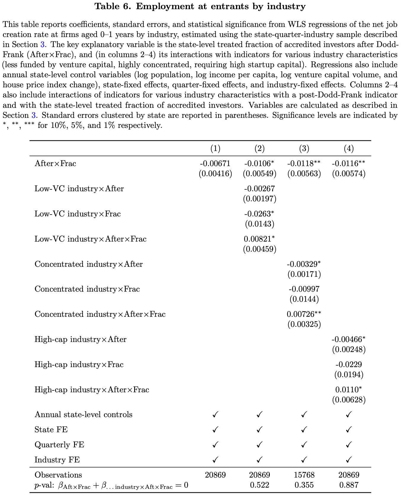
From Lindsey and Stein (2019 WP)
OLS and 2SLS with first stage and test statistics
Stata code
* This file will estimate the returns to college education using the "college in the county" instrumental variable
* which instruments for college attendance with whether there is a 2 or 4 year college near the respondent of the NLS.
* You will first need to install estout (ssc install estout), and you will need to pull the card data from my Mixtape
* in the cloud.

use "https://storage.googleapis.com/causal-inference-mixtape.appspot.com/card", replace

cap n tempvar tempsample
cap n local specname=`specname'+1
reg  lwage  educ  exper black south married   smsa
cap n estadd ysumm
cap n estimates store ols_`specname'

cap n local specname=`specname'+1
reg educ nearc4 exper black south married   smsa
cap n local biv = _b[nearc4]
cap n local seiv = _se[nearc4]
cap n unab ivs: nearc4
cap n local xlist: colnames e(b)
cap n local ivs: list ivs & xlist
cap n test `ivs'
cap n local F_iv=r(F)
cap n local specname=`specname'+1

cap n ivregress 2sls lwage (educ=nearc4) exper black south married   smsa, first
cap n estadd ysumm
cap n estadd scalar biv  = `biv'
cap n estadd scalar seiv = `seiv'
cap n estadd scalar F_iv = `F_iv'
cap n rivtest
n return list
cap n local ar_chi2=r(ar_chi2)
cap n local ar_p=r(ar_p)
cap n estadd scalar ar_chi2 = `ar_chi2'
cap n estadd scalar ar_p = `ar_p'
cap n estimates store tsls_`specname'

#delimit ;
	cap n estout * using ./card.tex,
		style(tex) label notype
		cells((b(star fmt(%9.3f))) (se(fmt(%9.3f)par)))
		stats(biv seiv F_iv ar_p N ymean ysd, star(biv)
		labels("College in the county" "Robust standard error " "F statistic for IV in first stage" "Anderson-Rubin test" "N" "Mean Dependent Variable" "Std. Dev. Dependent Variable")
			fmt(3 3 3 2 %9.0fc 3 3))
		keep(educ exper black south married smsa) replace noabbrev starlevels(* 0.10 ** 0.05 *** 0.01)
		title(OLS and 2SLS regressions of Log Earnings on Schooling)
		collabels(none) eqlabels(none) mlabels(none) mgroups(none)
		prehead("\begin{table}[htbp]\centering" "\scriptsize" "\caption{@title}" "\label{2sls_1}" "\begin{center}" "\begin{threeparttable}" "\begin{tabular}{l*{@E}{c}}"
"\toprule"
"\multicolumn{1}{l}{\textbf{Dependent variable}}&"
"\multicolumn{2}{c}{\textbf{Log wage}}\\"
"\multicolumn{1}{c}{}&"
"\multicolumn{1}{c}{OLS}&"
"\multicolumn{1}{c}{2SLS}\\")
		posthead("\midrule")
		prefoot("\\" "\midrule" "\multicolumn{1}{c}{First Stage Instrument}\\")
		postfoot("\bottomrule" "\end{tabular}" "\begin{tablenotes}" "\tiny" "\item Standard errors in parenthesis. * p$<$0.10, ** p$<$0.05, *** p$<$0.01" "\end{tablenotes}" \end{threeparttable} \end{center} \end{table});
#delimit cr
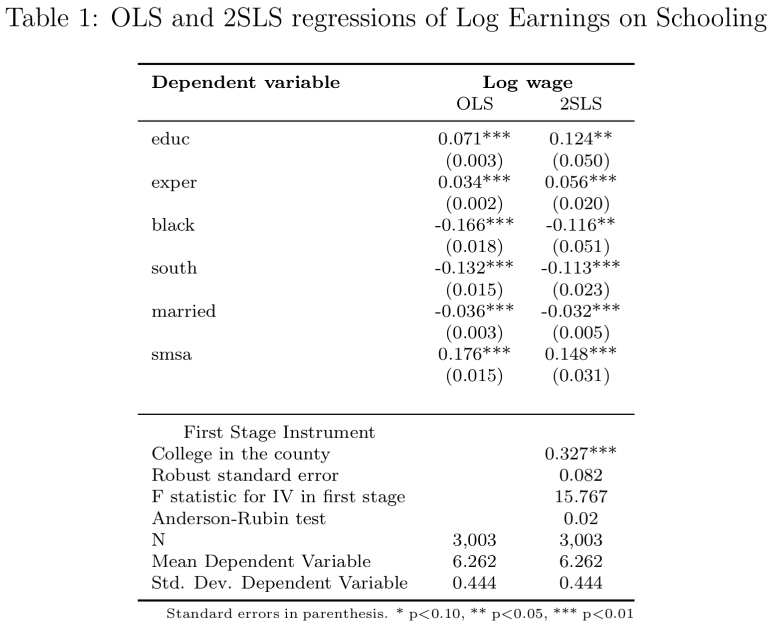
From "Causal Inference: The Mixtape" by Scott Cunningham
Summary statistics
Stata code
gen t_entry_norm1 = entry_norm1 * 100
label var t_entry_norm1	"Firm entry rate (\%)"

gen t_frac = frac * 100
label var t_frac	"Frac (\%)"

gen t_chHPI = chHPI * 100
label var t_chHPI	"House price index change (\%)"

eststo clear
eststo: quietly estpost summarize	t_entry_norm1 ///
									t_frac lnpop lnpercap lnvc t_chHPI ///
								if ${SAMPLEIF} & (age_buckets == 1) & (pa > 0), detail

esttab using "${OUTPATH}summstat_bds_sy.tex", replace ///
	cells("mean(fmt(2)) sd(fmt(2)) p50(fmt(2)) p25(fmt(2)) p75(fmt(2))") label booktab nonumber nomtitles
eststo clear
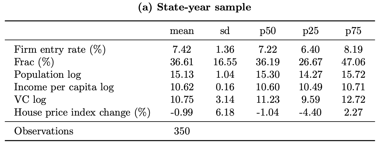
From Lindsey and Stein (2019 WP)
Summary statistics with added column
Stata code
label var responses		"Responses"
label var scams			"Scams"
label var nonscams		"Non-scams"
label var offers		"Offers"


estpost tabstat anyresponse anyscam anynonscam anyoffer [aw = stateweight], statistics(mean) columns(statistics)
matrix anys = e(mean)
matrix colnames anys = responses scams nonscams offers	// Get column in same rows as responses scams nonscams offers
matrix rownames anys = anys

eststo clear
estpost tabstat responses scams nonscams offers [aw = stateweight], statistics(mean sd p25 p50 p75 p95 max count) columns(statistics)

estadd matrix anys

esttab using "${OUTPATH}numberresponsesw.tex", ///
	cells("mean(fmt(a2) label(Mean)) sd(fmt(a2) label(Std.\ Dev.)) p25(fmt(a2) label(25\%)) p50(fmt(a2) label(50\%)) p75(fmt(a2) label(75\%))  p95(fmt(a2) label(95\%)) max(fmt(a2) label(Max.)) anys(fmt(a2) label(Frac.\ $>0$))") ///
	nostar nonumbers nomtitle label booktabs width(38em) replace
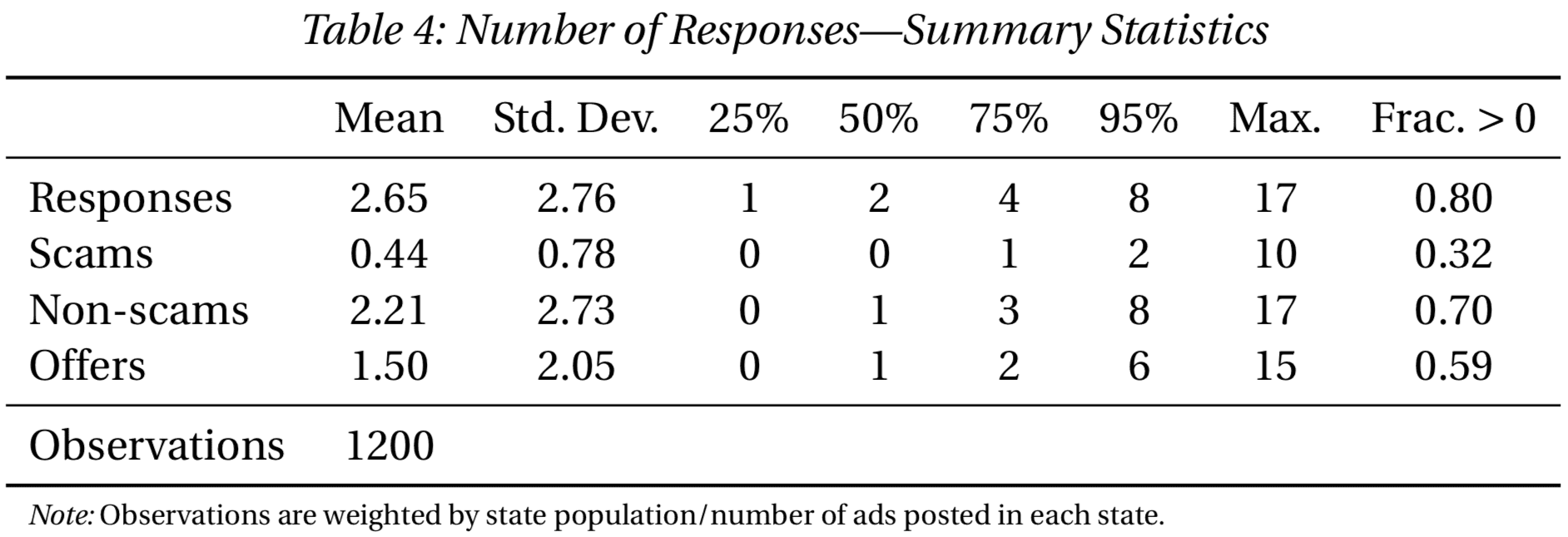
tabout
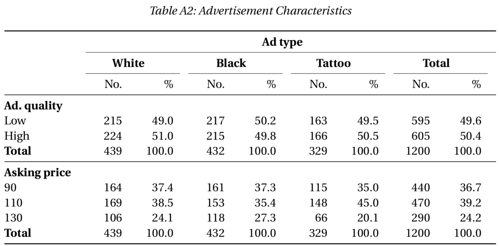
Two-way crosstabulation with percentages
Stata code
global ADCHARS			"highquality price"
label var highquality "Ad.\ quality"

tabout ${ADCHARS} type using ${OUTPATH}adchars.tex, c(freq col) f(0 1) ///
	cl1(2-11) cl2(2-3 4-5 6-7 8-9 10-11) topstr(Advertisement Characteristics\label{tab:adchars}|\textwidth) ///
	replace style(tex) bt font(bold) topf(top.tex) botf(bot.tex)
texdoc
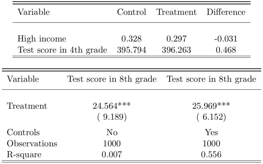
Covariate balance and regressions
Stata code
/**********************************************************************************************
* Title: Example for LaTeX output using texdoc
* Created by: M. Bennett
* Created on: 04/02/19
* Purpose: This dofile generates fake data and shows how to build different tables in LaTeX
			using texdoc
* Last Modified on: 04/02/19
* Last Modified by: MB
* Edits:
	[04/02/19]: Created dofile
**********************************************************************************************/

* Start with an empty dataset
clear

* Set a seed so results are replicable (I'm using Stata 15, just in case)
set seed 123

* Set number of obs
set obs 1000

* Generate an error term u normally distributed
gen u=rnormal(0,100)

* Generate a random treatment variable:
gen treat = runiform(0,1)>0.5
label var treat "Treatment"

* Generate a binary covariate (50% of the population)
gen x1=runiform(0,1)>0.7
label var x1 "High income"

* Generate a continuous covariate
gen x2=rnormal(400,110)
label var x2 "Test score in 4th grade"

* Generate an outcome:
gen y= 100 + 50*x1 + 1*x2 + 20*treat + u
label var y "Test score in 8th grade"

* Generate a simple covariate table (there are different ways to run this, but here's one):
foreach var of varlist x1 x2{
	* Run a regression (using , robust to account for heteroskedasticity)
	reg `var' treat, robust

	* Store whatever you want (in this case, we are going to save the means for each group and the difference)
	global m`var'_0: di %6.3fc _b[_cons]
	global m`var'_1: di %6.3fc _b[_cons] + _b[treat]
	global dif_`var': di %6.3fc _b[treat]

	* Store the label of the variable, because it's easier then to put it in the tables:
	global lbe_`var' : var label `var'

	* Because I also want to know if the difference is significant, I'm going to store the p-value (and the star level)
	qui test treat=0
	global p_`var': di %12.3fc r(p)
	glo star_`var'=cond(${p_`var'}<.01,"***",cond(${p_`var'}<.05,"**",cond(${p_`var'}<.1,"*","")))
}

* Now, lets generate our balance table! (heads up, if you haven't set a current directory (cd), it's going to store this table wherever is the default).
* PS: It's not necessary to do this with a loop, but if you have a lot of covariates, might be useful.

texdoc init balance_table.tex, replace force
tex \begin{tabular}{lccc} \toprule \toprule
tex Variable			& 	Control	& Treatment & Difference \\
tex \addlinespace \hline \\
foreach var of varlist x1 x2{
tex ${lbe_`var'} & ${m`var'_0} & ${m`var'_1} & ${dif_`var'}${star_`var'}\\
}
tex \hline \hline
tex \end{tabular}

texdoc close


* Let's run a regression now! (with and without controls)

global covs0 "treat"
global covs1 "treat x*"

global lbe_y : var label y
global lbe_treat : var label treat

forvalues spec=0(1)1{

	*Run the regression
	reg y ${covs`spec'}, robust
	*Save some outputs
	scalar N=e(N)
	scalar r2=e(r2)
	global N_`spec'=N
	global r2_`spec': di %6.3fc r2

	*Store the variable of interest
	global b_`spec': di %6.3fc _b[treat]
	global se_`spec': di %6.3fc _se[treat]

	qui test treat=0
	global p_`spec': di %12.3fc r(p)
	glo star_`spec'=cond(${p_`spec'}<.01,"***",cond(${p_`spec'}<.05,"**",cond(${p_`spec'}<.1,"*","")))
}


texdoc init treatment_effect.tex, replace force
tex \begin{tabular}{lcc} \toprule \toprule
tex Variable			& 	${lbe_y}	& ${lbe_y} \\
tex \addlinespace \hline \\
tex ${lbe_treat} & ${b_0}${star_0} & ${b_1}${star_1}\\
tex 			& (${se_0}) & (${se_1})\\ \addlinespace
tex Controls & No & Yes \\
tex Observations & $N_0 & $N_1 \\
tex R-square & $r2_0 & $r2_1 \\
tex \hline \hline
tex \end{tabular}

texdoc close
From Magdalena Bennett
Note
I created this page in response to Twitter discussions suggesting there’s interest in learning more about the wide range of techniques researchers use to work with Stata and LaTeX. I also wanted to learn more about how to use github (where this page is hosted).
Please feel free to suggest additions, either by submitting pull requests to the github respository (if you know how to do so), or by contacting me directly.